It is well known that acceptance criteria for validation in the field of pharmaceutical industry is very strict, to ensure product excellence. Therefore, the design of environmental and process equipment must be performed in a way that makes sure that results will stay within a very narrow deviation range.
When we face complex problems such as:
- Temperature distribution on a certain volume or surface, such as a room or a heat sink
- Airborne particle patterns in a room
- Air velocity magnitude at certain point within a room or a pipe
- Cold surfaces generating condensation on a chamber wall or pipe
- Radiation effect inside a vacuum chamber
- Forces and stress generated by pressure or flow velocity against a solid part
Using trial-error and prototyping is only feasible when time and budget is available
We must choose one (or a combination of) methods to solve the problem:
1. Trial-error, prototyping, empiric methods and experience
2. “Hand” calculations using formulas, tables, charts, and coefficients
3. Computational Fluid Dynamics
Using trial-error and prototyping is only feasible when time and budget is available, normally for serial product but not for short delivery special equipment. Additionally, it is always better to perform first stages of design with CFD and let prototypes be used for a second stage of the project, when the main decisions have already been made.
Using hand simple or differential calculations using formulas, tables, coefficients, and charts, is a tedious process which is often unreliable and incomplete. For instance, if we try to forecast the internal temperature of a convoluted ventilated heat sink by using a “manual” calculation method, we will spend a huge amount of time. Afterwards, the results will not be reliable enough to provide a definite answer. A huge safety margin will then need to be included, and the final product will not be considered ‘optimum’. Empiric tables, charts and coefficients will help us, but only few simple cases are registered in bibliography.
For these reasons’ old methods of assay-error and hand calculations have been replaced by a powerful initial analysis supported by computerised calculation. This method is fast, comprehensible, reliable, and cost effective. It is not by chance that the most challenging designs are using CFD: aerospace, microelectronics, rotating machinery, or even improving performance of racing F1 cars or ultra-fast sailing boats.
The computer applies Navier Stokes equations
How is a CFD study performed?
Step 1: 3D MODEL. An accurate 3D model containing all the solids and fluids involved in the study is needed. As a rule, we could affirm that the better the 3D precision is, the more reliable the results of the CFD will be.
But it must also be considered that very small details in the model will make further steps tedious and even unfeasible. Therefore, small details not relevant for the aim of the study can be simplified or even suppressed.
Step 2: MESH. The aim of meshing is to divide fluid and solid volumes into very small pieces (finite elements).
Size of elements can be automatically or manually adapted to geometry. For instance, we can accept to have medium sized air elements at the centre of a room, but we need to make them smaller at the proximity of a diffuser or exhaust grid, where air is supposed to move and rotate in a more turbulent way.
Step 3: BOUNDARY CONDITIONS. At this step all known perimetral conditions must be introduced. For instance, surfaces where a fluid is entering or exiting our volume (grids or filters), as well as related velocity or volumetric/mass flow rate at these areas. Other typical conditions to be defined are walls, isolated walls, openings, or constant temperature areas.
Step 4: CALCULATION. This stage is the real core of the CFD study. The computer applies Navier Stokes equations as well as mass and energy conservation principles between all the finite elements defined in the meshing step.
Once the temperature, pressure, velocity, and other variables of all elements have been calculated, the process starts again. Each round is called iteration. At this point the software often offers a graph showing how error becomes smaller iteration after iteration. When results become stable, the calculation is finished. It must be said that there are two main types of calculation:
Steady state: The calculation looks for an equilibrium scenario, where mass and energy in all our domain is balanced. It gives us a static “picture” of the conditions when equilibrium is reached.
Time dependent: A small time increase is applied after each iteration, and all these transient results are stored. At the end of the whole process, we can observe the evolution of conditions along time. This type of calculation can generate clips or videos showing real time or accelerated evolution.
Step 5: RESULTS. Once the calculation is finished the computer has stored the value of dozens of parameters at each single element (and at each single time moment in case of time dependent study).
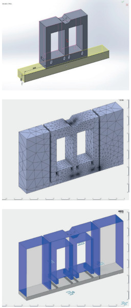
Steps 1-3 in a CFD study
Therefore, several ways of showing these values are often available in the software.
Sections: Once a section is defined all the mesh elements cut by this section are coloured depending on the selected variable and specified colour legend. Surfaces: Like sections but applied to existing surfaces in our model. Vectors: Arrows showing direction and magnitude of velocity at all mesh elements cut by a section or present in a surface. Streamlines: They show the trajectory followed by a fluid. Article path: Trajectory of particles thrown in a fluid. Some software allows to configure particles in terms of material and size. Isosurfaces: Surfaces in which a parameter has got the same value Calculated values: Just an average, maximum or minimum value in a certain point, surface, or volume.
Real case examples
Freeze drier sight glass condensation avoidance. Challenge: When the freeze dryer chamber is at its lowest temperatures there is a risk of the chamber’s external surfaces cooling down too much. If the room has got a certain ambient humidity, then condensation may occur. The risk is focused on the sight glass, as it is one of the few parts of the chamber which cannot be thermally insulated easily. Analysis: A simulation was performed considering internal chamber temperatures at about -80ºC in presence of air and later with only vacuum inside. The worst-case scenario was in presence of air due to conduction and convection. The output of the simulation was the temperature mapping at the external surfaces of the sight glass. This allowed us to determine whether condensation was going to take place or not. Actions: Determine limit conditions in which condensation was proven and look for thermally improved sight glass.
Ethylene Oxide sterilisation pre-conditioning and aeration chambers optimisation. Challenge: How to improve thermal and gas exchange between solid product and ventilation hot air into product pre-conditioning and aeration chambers. Analysis: Many different supply and return hot air patterns were configured into the room. Analyse to determine which patterns generate a quicker and more homogeneous heating up of product. Temperature of product surfaces and internal temperature of product during this time was used as an indicator to compare options. Second stage was to define many different flow rates and find out the best energy consumption Vs thermal performance balance. Actions: Supply nozzles and return grids placed following the best CFD results. Air flow rates adjusted to the best-balanced configuration.
Laminar flow performance into a grade a room. Challenge: How to optimise location of return grids and physical barriers in grade A laminar flow room. Analysis: A complete grade A room, containing a filling line was simulated as a combination of descending laminar flow and turbulent flow (part of the room was grade B). Once return grids were placed in the best possible locations, the air flow rate of each grid was adjusted individually to make air patterns regular and relaxed all around the perimeter. This adjustment is the same that will be performed later at site using manual regulation dampers. Actions: Position of return grids were optimised and airflow rate per grid was defined in advance.
Floor condensation avoidance. Challenge: Preconditioning room with very high absolute humidity rate presents risk of condensation due to low temperature of concrete floor in winter. If the temperature of the floor stays below preconditioning room’s dew point condensation will occur. Analysis: Many different configurations in terms of floor insulation and thermal bridge breakdown have been simulated considering worst case scenario, which means high humidity within room and low temperature at terrain below concrete slab. The results show that, in case of no insulation, some area in the floor stays below dew point. Problem is completely solved after applying floor insulation. Other intermediate solutions were also simulated. Actions: Establish air and ground conditions above which condensation is going to occur. In case that these conditions are overpassed then recommend floor insulation.
Air flow performance in a downflow booth. Challenge: How to optimise laminar flow and containment generated by standard range of downflow booths. Analysis: The complete standard range of downflow booths were analysed. Return grids dimension and percentage of bleed air, as well as different type of side and front enclosures were simulated and calculated. Side and front air knives to replace PVC curtains were also analysed. Airborne particles were virtually thrown into the study, so it was possible to simulate particle counting to evaluate the performance of several different configurations. Actions: Dimension and velocity in return grids and amount of bleed air were adjusted to obtain the best possible performance. It was also possible to establish the buffer zone area (not safe zone in terms of containment and product protection) in case of removing front or side PVC stripped curtain.
Air flow performance below an operating theatre canopy. Challenge: See how temperature of supply air influences the laminar flow pattern and forecast which will be the velocity on the operating field above the patient. Analysis: Operating theatre canopies are often enclosure-free. Therefore, the edge of the laminar flow must be carefully studied to detect possible room air entrance at the perimeter. The temperature difference between room and supply air is the main parameter which will define how protected the perimeter is against external particles. Actions: Generate knowledge about how temperature difference affects laminar flow protection, and determine design recommendations accordingly.
Forecasting with high precision was inconceivable just few decades ago
Conclusion
The use of Computational Fluid Dynamics to optimise performance of high-tech equipment and installations is proven to generate very significant increases in quality and efficiency. The fact that we can forecast, with high precision, the behaviour of fluids and solids exposed to complex physical phenomena was inconceivable just few decades ago. Therefore, a tremendous opportunity has evolved, and we the engineers and the final users are compelled to investigate and explore this tool to achieve maximum result now and in the future.